Research

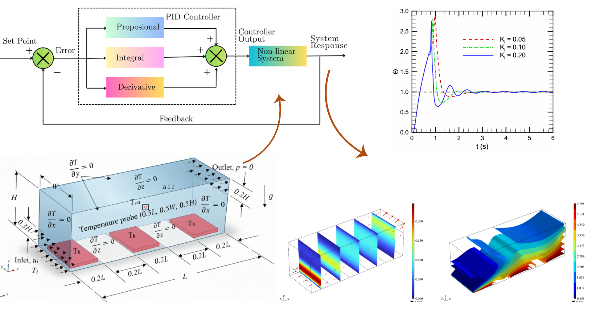
Employing the control law to regulate convection can provide an optimal system for many sophisticated applications, such as MEMS fabrication, electronic component cooling, and drug manufacturing facilities. A computational approach is always advantageous in this regard for affordable trial and error. A more advanced version of this can be established by creating a digital twin for the application. Other improvements include the selection of appropriate controllers with tunable parameters for the system, the insertion of multiple sensors in the domain, and the acquisition of precise measurements. Another is quantifying the uncertainty and using its thresholds (mean and variance) during feedback. The precision control needs integration with advanced data analysis in real-time and statistical methods to fully capture the system's (spatio-temporal) dynamics.

Below is a related published work of mine (Deb et al., 2023^†), in which active flow control was implemented for a thermal system. This was done through computation and can be leveraged for many advanced applications with the aforementioned improvements.

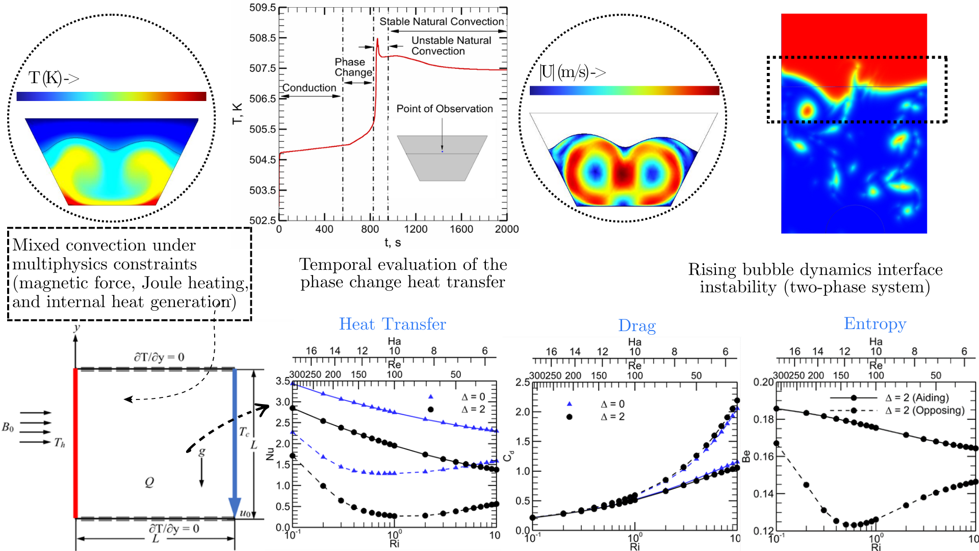
The transport of scalar or vector quantities with fluid flow creates strongly coupled dynamics, where nonlinear interactions between terms like forces, energies, and fluxes complicate the analysis. Such multiphysics-constrained flows are ubiquitous in thermofluidics, fluid–structure interaction, reactive flows, magnetohydrodynamics (MHD), and electrohydrodynamics (EHD). Although analytical and semi-analytical models can suffice for simplified flows, they have limited applicability. High-fidelity (multiscale/fieldscale) simulations based on numerical methods (FDM, FEM, FVM, SEM, LBM) have proven strengths in computational science. Yet, computation often struggles to select the just method with right discretization schemes (reparameterization, adaptive meshing) and time stepping (explicit or implicit). Meanwhile, this should also complay with stability and convergence, as well as overall run-time efficiency. Multiphase and phase-change flows require additional modeling with phase-field, level-set, and volume-of-fluid methods to track interfaces. To lower computational costs and improve efficiency, machine learning (ML), deep learning (DL), probabilistic surrogates, and reduced-order modeling (POD, DMD) are becoming popular. The field is evolving from purely data-driven methods to physics-informed and operator learning frameworks. It is possible to integrate a learnable model with existing physics and solvers, or even replace parts of them entirely. This choice is opening new frontiers. Increasingly, scientific machine learning (SciML) and differentiable physics are being applied to this class of problems (multiphysics flow) for more efficient forward simulations and inverse estimations.

Related publications:

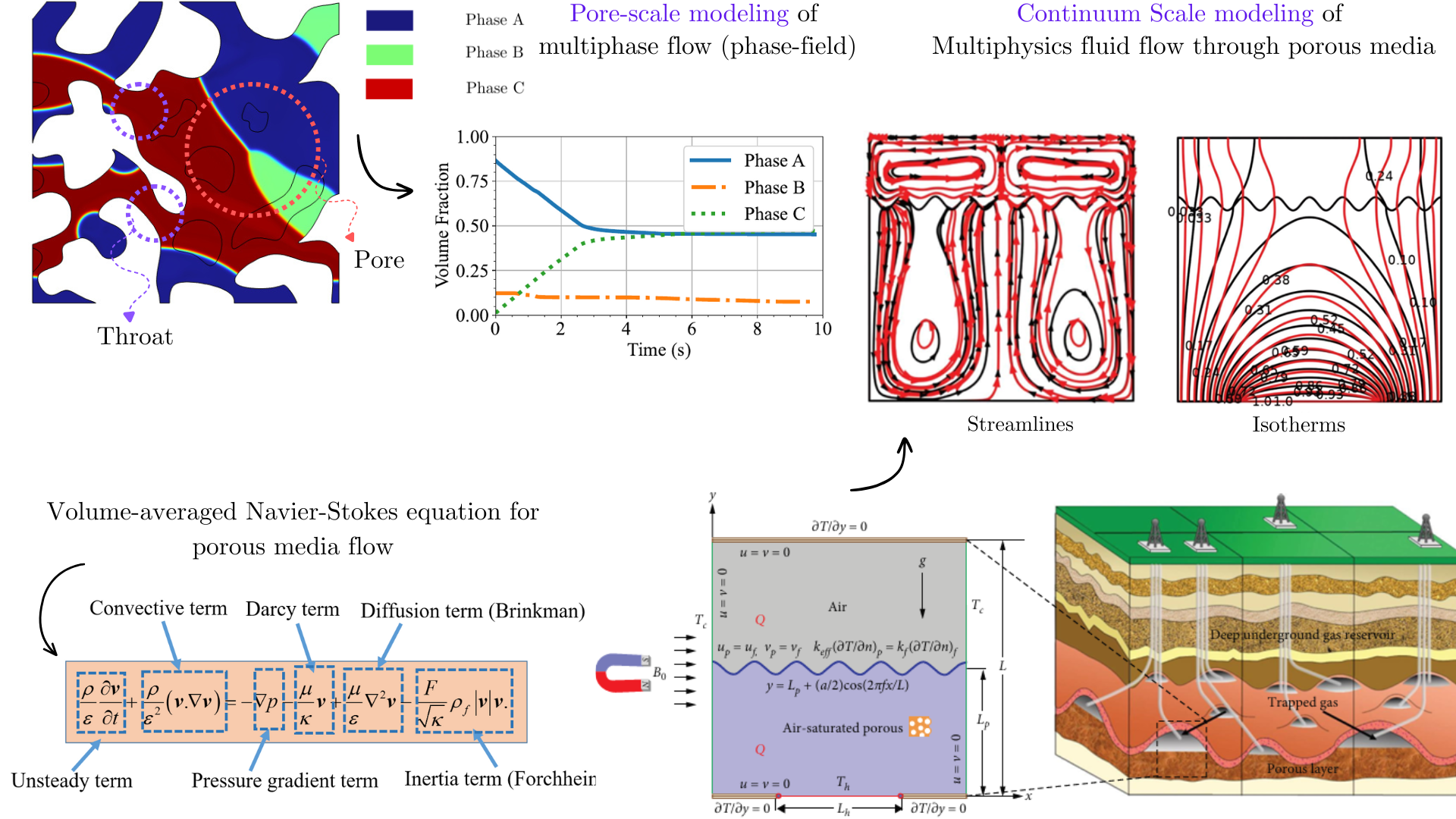
Flow through porous media involves a complex flow path for the intended fluid, which can vary widely in scale. Methods allow for characterizing flows from the microscale (pore-scale modeling) to the continuum (volume averaging). The momentum balance captures creeping, viscous, inertial, or diffusive effects. Darcy’s law forms the basis for creeping flow (low Reynolds number) with negligible inertial effects. This law has been modified by Brinkman, who accounts for viscous diffusion (shear near boundaries), and Forchheimer, who considers inertial effects during high-velocity flows. Common applications include subsurface flow modeling, such as in aquifers and reservoirs. Subsurface flow has some unique features. The heterogeneity and anisotropy of porous media, as well as additional interactions from geomechanics, chemical kinetics, or heat transfer, are just a few examples. Multiphase and multicomponent flows with larger spatial and temporal scales make this flow type challenging to study. On top of that, fluids behave quite differently in their supercritical states, where large changes in density, compressibility, and transport properties occur. A single diffusivity equation that combines the continuity, momentum, and equation of state can adequately describe this behavior. This knowledge is extensively used in well testing for reservoir engineering, aquifer pressure responses, carbon dioxide sequestration, and geothermal systems.

Related publications:

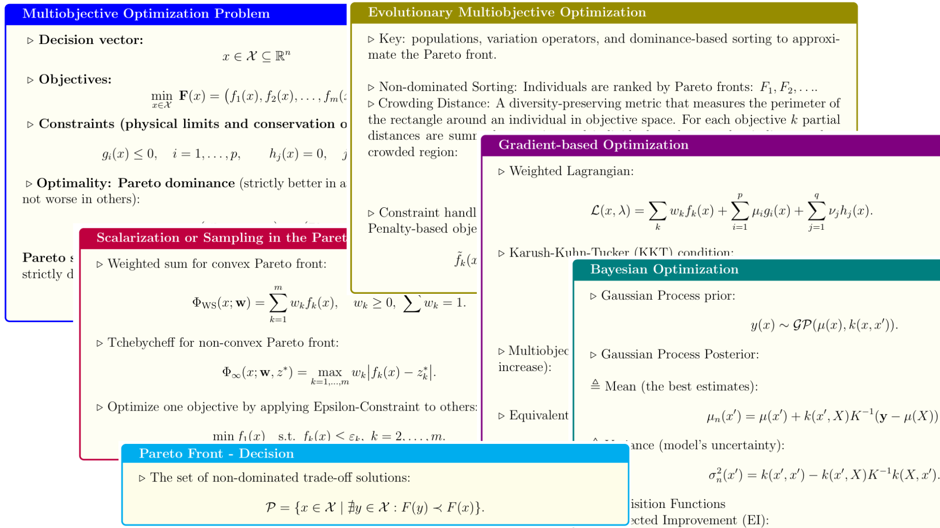
For an optimization task, a system is considered complex when it involves many decisions or design variables, often with multiple objectives. The objective may be to reduce costs (materials) or to improve performance, efficiency, or robustness in the face of highly nonlinear relations, high-dimensionality, and interdependence. These features are common in real-world engineering problems. Several physical limits (inequality constraints) and conservation of quantities (equality constraints) must also be weighed for true optimality. A defined mathematical model or closed-form solution is required for the analytical approach to work. The gradient-based algorithm can quickly find a solution for a smooth and differentiable function with clearly defined extrema (local; global only for convex functions). However, the method struggles with increased dimensionality or it may not work for nonconvex functions. This can be overcome with adaptive gradients or surrogate-based or data-driven methods that are robust and have much lower computational costs. It is also established that objective functions are not always analytic or may lack a defined mathematical expression for gradient evaluation. In those cases, Bayesian optimization (with uncertainty) can still work. Metaheuristic algorithms (such as genetic, differential evolution, particle swarm) are even more powerful because they are global in nature and work well with stochastic objectives. A simple set of rules (mutation, crossover, and selection) eliminates the need for gradient information. This is a key advantage for many optimization tasks.

Please find a recent work ^† of ours, where the population-based metaheuristic algorithm is used for an advanced thermodynamic application (optimization task).

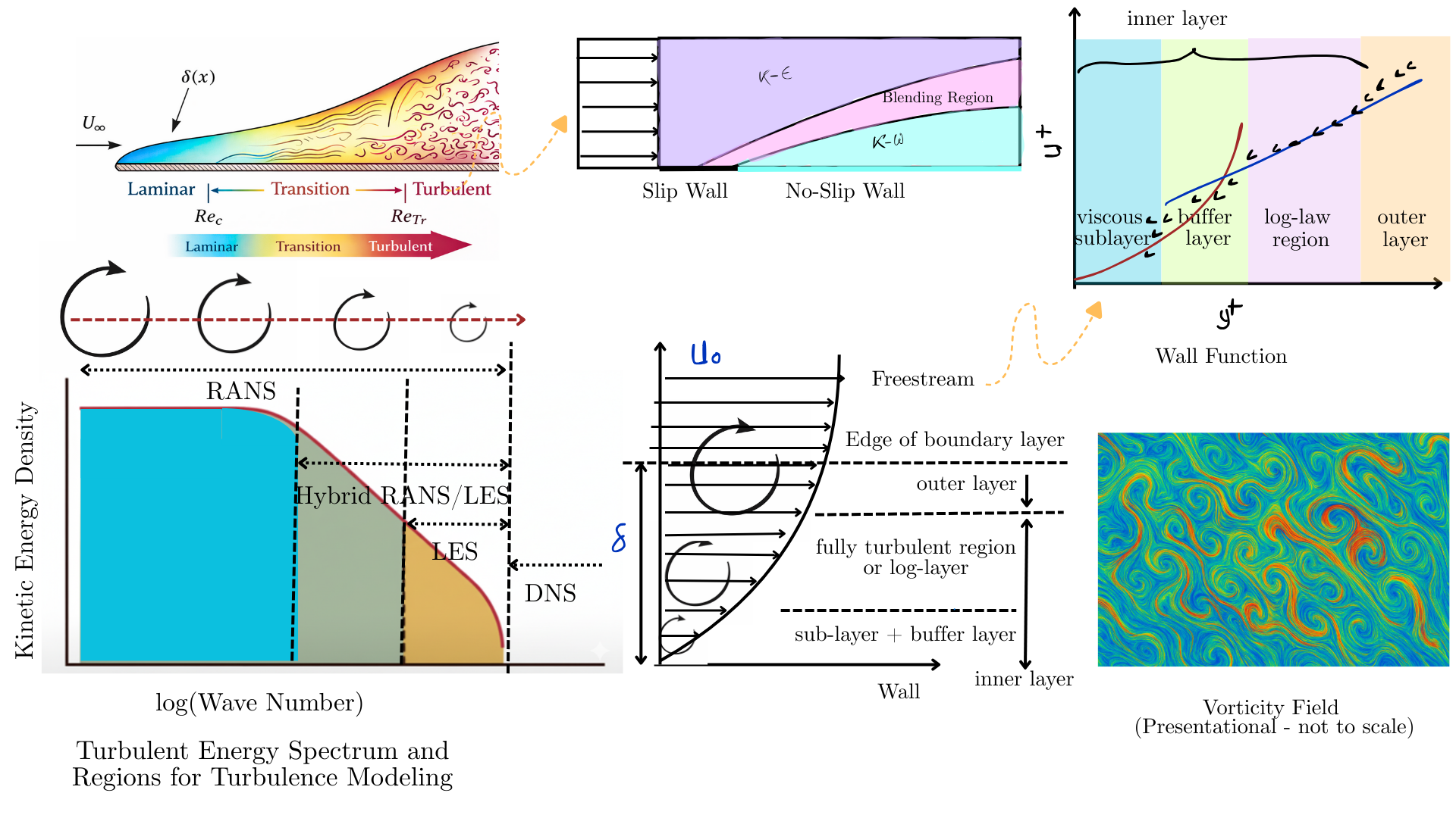
“At moderate Reynolds numbers, the restraining effects of viscosity are too weak to prevent small, random disturbances in a shear flow from amplifying. The disturbances grow, become non-linear, and interact with neighboring disturbances. This mutual interaction leads to a tangling of vorticity filaments. Eventually the flow reaches a chaotic, non-repeating form describable only in statistical terms. This is turbulent flow.” - Launder, B. E., An Introduction to the Modeling of Turbulence, VKI Lecture Series 1991-02, March 18-21, 1991.

Turbulence is the limit of computational fluid dynamics (CFD), as no level of computational power can achieve the desired accuracy. Turbulence contains a wide range of energy spectra, from production to inertial to the dissipation range. A regular flow (laminar) subjected to external disturbances in its free stream (acoustic waves, transported vorticity from upstream, or changes in pressure, density, or temperature), surface roughness, or the motion of a body causes instability in the shear layer. Statistical measures (mean, variance) can quantify turbulence but omit the full range of length and time scales. Turbulent kinetic energy, dissipation rate, and kinematic viscosity define the largest (energy-producing) to the smallest (Kolmogorov) scales in the flow. Modeling turbulence essentially dictates which turbulence scales can be modeled and which need to be resolved on a computational grid by solving the unsteady Navier-Stokes equations. DNS requires no modeling, since all scales are resolved on the grid by making the grid scale comparable to the Kolmogorov length scale. However, with such finer details, computational cost increases exponentially, which ultimately restricts DNS for complex geometries with non-uniform grids and high-Reynolds-number flows. Conversely, the Reynolds-averaged Navier-Stokes (RANS) equations model the entire range as a single length scale in a statistically steady sense. RANS models include algebraic models, one-equation models (Spalart-Allmaras), and two-equation models (k - ε and k - ω), which are based on eddy viscosity or shear stress transport (SST). No single model fits the entire computational domain; for example, k - ω captures near-wall phenomena well, while k - ε performs better in free-stream regions. Large Eddy Simulation (LES) requires modeling the smallest approximately 20% of the scales (subgrid scales), while resolving the rest on computational grids. LES takes advantage of the isotropic nature of turbulence at its lowest scales, and spatial filtering allows integration of a subgrid-scale model (e.g., the Smagorinsky model). Another efficient solution is to use RANS for the boundary layer and LES away from it, e.g., hybrid RANS/LES turbulence modeling. As a standard, all models are calibrated against experiments or DNS.

Related work: